
The questionnaires are back. There are two hundred and thirty of them in a nylon bag, SPSS is open on a borrowed laptop, and the cursor is blinking in an empty grid. This is where most Nigerian project groups lose a week — not to the statistics, which are usually simple, but to not knowing the order of operations.
What follows is that order, in nine steps, with the exact menu path for every procedure an undergraduate project needs. Paths are quoted as documented in Kent State University Libraries’ freely available SPSS tutorials; recent versions keep them stable, but if a menu on your machine reads slightly differently, trust your machine.
Two things belong upstream of this guide. You should already know which tool answers which research question — that decision is made in choosing the statistical test for your project, not in the software. And what you do with the output afterwards is a separate skill, set out in writing Chapter Four.
Step 1: Number the questionnaires before you touch a computer
Output: a physical stack in which every usable copy carries a unique case number.
- Separate the incomplete copies into their own pile. Count both piles and write both counts down; your return rate needs them.
- Write 1, 2, 3 in the top corner of each usable questionnaire.
- Keep the stack in that order for the whole encoding session.
This takes fifteen minutes and it is the only thing that makes an encoding error recoverable. When SPSS later shows a respondent aged 220, the case number tells you which sheet of paper to check. Without it you are re-reading 231 questionnaires to find one typo.

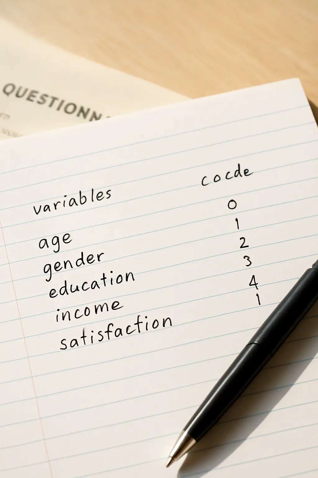
Step 2: Build the variable list before entering a single response
Output: a complete Variable View, filled in before any data exists.
Click the Variable View tab at the bottom of the data editor. Every questionnaire item becomes one row, and four columns matter.
- Name — short, no spaces, systematic. Use
sex,level,dept, thenB1toB10andC1toC10so the names mirror the sections of your instrument. - Label — the full item text. This is what prints on your output tables, so a good label here saves retyping every row of Chapter Four by hand.
- Values — the numeric code for each option: 1 = Strongly Disagree through 4 = Strongly Agree, or 1 = Male, 2 = Female.
- Measure — Nominal for categories such as sex or department, Ordinal for Likert items, Scale for genuinely continuous variables such as age or a computed total.
Getting Measure right early prevents a whole class of later confusion, because SPSS uses it to decide which procedures it offers you for a variable.
Step 3: Encode the responses, one row per respondent
Output: a Data View grid with as many rows as you have usable questionnaires.
Switch to Data View and work down the numbered stack. One respondent is one row; one item is one column. Never put two respondents on one row and never spread one respondent across two.
Three rules prevent the expensive mistakes. Leave a genuinely unanswered item blank rather than typing 0 — zero is a real value and it will drag your mean down. Decide as a group how to treat an item where a respondent ticked two boxes, then apply that decision to every case rather than case by case. And if you split encoding across several laptops, agree the codebook in writing first, because merging three files that coded sex differently costs more than the encoding did.
Save as a .sav file after every fifty cases, with the date in the filename.
Step 4: Reverse-score the negatively worded items
Output: new variables in which every item points the same direction.
If your instrument contains an item like “Power supply has no effect on how long I study”, a high score there means the opposite of a high score on the rest of the scale. Averaging it in unreversed will depress your grand mean and wreck your reliability coefficient.
- Go to Transform > Recode into Different Variables.
- Move the negatively worded item across and give the output variable a new name, such as
B7r. - Click Old and New Values and enter the reversal for a four-point scale: 1→4, 2→3, 3→2, 4→1.
- Click Add for each pair, then Continue and OK.
Always recode into a different variable, never over the original. Keeping the raw column means a mistake here is one recode away from being fixed rather than a re-encoding away.
Step 5: Screen the data before you analyse it
Output: a frequency table for every variable, checked against the range each is allowed to take.
Run Analyze > Descriptive Statistics > Frequencies, move all your variables across, and read the output for three things.
- Impossible values. A four-point item with a maximum of 5 is a typo. Find the case number and check the paper.
- Missing counts. Every variable’s Valid N should equal your analysed N unless you know why it does not.
- Category totals. The frequencies for sex should sum to your N. If they do not, a case is miscoded.
Fix everything you find here before running anything else. An error corrected now costs a minute; the same error found after three tables are written costs the afternoon.
Step 6: Run the reliability analysis
Output: a Cronbach’s alpha for each section of your instrument.
- Go to Analyze > Scale > Reliability Analysis.
- Move in the items of one section only — Section B on its own, then Section C on its own. A scale measuring two different constructs is not one scale.
- Leave the Model on Alpha.
- Click Statistics and tick Item, Scale, and Scale if item deleted.
- Read the alpha, then read the “Cronbach’s Alpha if Item Deleted” column to see whether one bad item is dragging the section down.
Report the coefficient with the number of items and the pilot sample it came from, in Chapter Three. You will be asked at the defence which software produced it, so do not report a figure you did not compute.
Step 7: Produce the descriptive tables Chapter Four needs
Output: the bio-data table and the per-item mean tables, in that order.
For the respondent profile — sex, level, department — use Analyze > Descriptive Statistics > Frequencies and take the frequency and percentage columns straight into your table.
For the “level of” or “extent of” research questions, use Analyze > Descriptive Statistics > Descriptives with the Likert items of that section selected; the Mean and Std. Deviation columns are exactly what your table needs. For the grand mean, build a computed variable first with Transform > Compute Variable using the MEAN function across the items of that section.
Compare each mean against your criterion mean — 2.50 on a four-point scale — and fill the Decision column accordingly.
Step 8: Run the inferential test each hypothesis needs
Output: one output block per hypothesis, and no blocks you cannot attach to a hypothesis.
| What your hypothesis asks | Procedure | Menu path |
|---|---|---|
| Are two categorical variables associated? | Chi-square test of independence | Analyze > Descriptive Statistics > Crosstabs, then Statistics > Chi-square |
| Are two scale variables related? | Pearson correlation | Analyze > Correlate > Bivariate |
| Are two ordinal or non-normal variables related? | Spearman’s rho | Analyze > Correlate > Bivariate, tick Spearman |
| Do two groups differ? | Independent-samples t test | Analyze > Compare Means and Proportions > Independent-Samples T Test |
| Do three or more groups differ? | One-way ANOVA | Analyze > Compare Means > One-Way ANOVA |
| Is the distribution normal? | Shapiro-Wilk and Kolmogorov-Smirnov | Analyze > Descriptive Statistics > Explore, then Plots > Normality plots with tests |
Three details the dialogs will force on you. In Crosstabs the chi-square statistic is not produced unless you tick it under Statistics — the crosstab alone is only a contingency table, and this is the single most common reason a Nigerian student cannot find their chi-square value. In Bivariate, Pearson is selected by default and the test is two-tailed by default, with significance flagged at the .05 and .01 levels. And the Independent-Samples T Test will not run until you click Define Groups and specify the two codes being compared.
Step 9: Save the output and reconcile it before writing
- Save the data as
.savand the output as.spv, both dated, and copy both to a second device or a cloud folder. - Check that the Valid N on your output matches the analysed N you stated in Chapter Three.
- Check that every research question and hypothesis has exactly one output block, and delete the exploratory runs you did along the way.
- Check that the tools that produced your output are the ones you named in Chapter Three. If you changed one, change the chapter too.
Only then start writing. A Chapter Four built from unreconciled output will contradict Chapter Three somewhere, and that contradiction is the first thing a panel finds — as the standard question list in what is asked during a project defence makes clear. How the analysis chapter sits within the whole document is summarised in how many chapters a final year project has.
You have the output. Now write the chapter.
Tesify holds your chapters in the structure your department expects and keeps every citation attached to a source you actually opened, so the week after analysis goes into interpretation rather than formatting. Over 9,000 students have used it to write more than 15,000 chapters, and every word is still written by you.
Frequently asked questions
How do I analyse my project data using SPSS?
Number the questionnaires, build the full Variable View before entering data, encode one row per respondent, reverse-score the negative items, then screen with Frequencies. Only after screening do you run reliability, descriptives and your inferential tests.
What is the menu path for Cronbach’s alpha?
Analyze > Scale > Reliability Analysis, with the Model left on Alpha. Enter one section at a time and tick “Scale if item deleted” under Statistics to see which item is weakening it.
Why is my chi-square value not showing?
Because it is not produced by default. Open the Statistics button inside the Crosstabs dialog, tick Chi-square, then run it again.
How do I encode a four-point Likert scale?
Set the item’s Measure to Ordinal and define its Values as 1 to 4 with the verbal label attached to each number. Then type only the numbers into Data View.
Should I enter 0 for an unanswered item?
No. Leave it blank. Zero is a real value on a numeric variable and it will pull the mean down and misstate the count of valid responses.
Do I have to reverse-score negative items?
Yes, if you are averaging items into a section score or computing a reliability coefficient. Skipping it is the commonest cause of an unexpectedly low Cronbach’s alpha in an otherwise sound instrument.
How do I get the grand mean in SPSS?
Build the section score first with Transform > Compute Variable using the MEAN function across that section’s items, then run Descriptives on the new variable.
Which SPSS version do I need?
Any recent version handles everything an undergraduate project needs. Menu wording shifts slightly between releases, so state in Chapter Three the version you actually used rather than copying a number from another project.
My groupmates encoded on separate laptops and the files will not merge. What now?
Compare the Variable View of each file side by side before merging. Mismatched variable names, different codes for the same answer and different Measure settings are the usual culprits, and all three are fixable in the file that deviates rather than by re-encoding.
Do I keep the output file after the defence?
Keep it until your project is finally approved and bound. Panels ask to see output, corrections can require reruns, and rebuilding a lost analysis from paper questionnaires under deadline is a miserable weekend.
Can I do all of this without SPSS?
Yes. Free packages cover the same undergraduate procedures, and spreadsheets handle means and percentages. Whichever you use, name that one in Chapter Three rather than naming SPSS by habit.